Code
library(dplyr)
library(timeDate)
library(gg3D)
library(plotly)Taking advantage of the web format, here I show an interactive version of this figure.
library(dplyr)
library(timeDate)
library(gg3D)
library(plotly)We filter the data so they are all within 0.25 decimal degrees of the mean location of all points (I know, I know… decimal degrees are terrible, but the point here is the time dimension, not the geographical coordinates).
taxis <- read.table('taxis100.txt', sep=',') |>
rename(id = V1, t = V2, lon = V3, lat = V4)
lon.mean <- mean(taxis$lon)
lat.mean <- mean(taxis$lat)
taxis.bj <- taxis |>
mutate(time = as.double(timeDate(t))) |>
filter(abs(lon - lon.mean) < .25,
abs(lat - lat.mean) < .25)plotly makes a nice interactive plot, without too much fuss.
plot_ly(group_by(taxis.bj, id),
x = ~lat, y = ~lon, z = ~t, color = ~id,
type = 'scatter3d', mode = 'lines', asp = 1, lwd = 0.5)And more like the plot in the book, here is a static 2.5D version, using gg3d::stat_3D.
ggplot(taxis.bj, aes(x = lon, y = lat, z = time, group = id, color = id)) +
stat_3D(theta = 30, phi = 5, geom = "path",
alpha = 0.25, linewidth = 0.35) +
scale_color_viridis_c() +
axes_3D(theta = 30, phi = 5) +
coord_equal() +
theme_void() +
theme(legend.position = "none")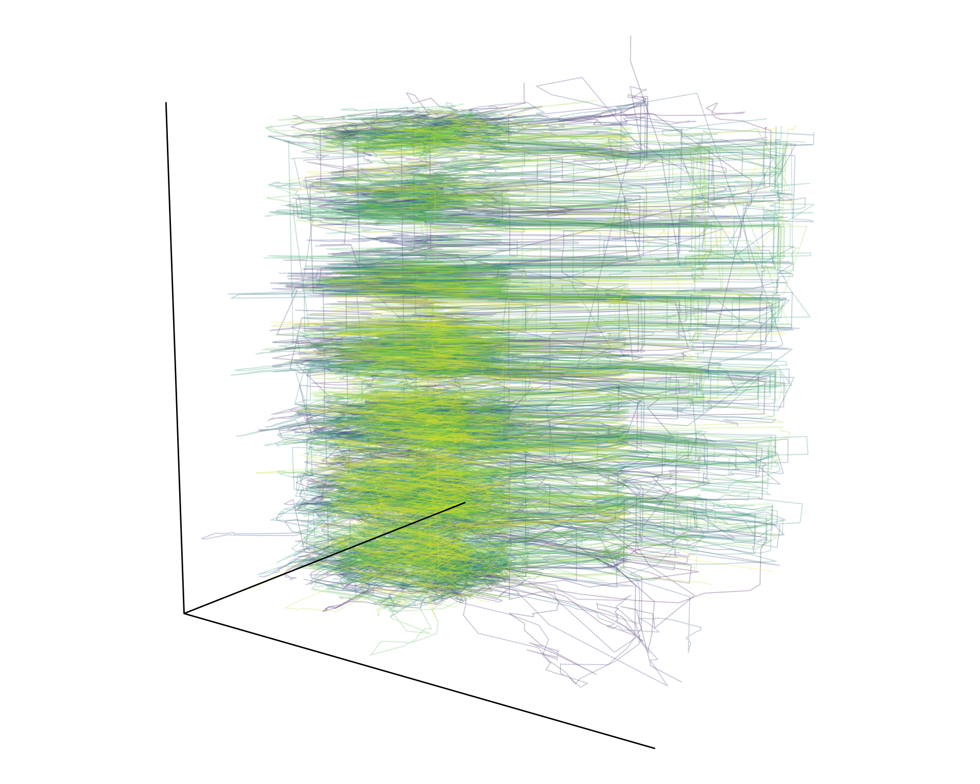
# License (MIT)
#
# Copyright (c) 2023 David O'Sullivan
#
# Permission is hereby granted, free of charge, to any person
# obtaining a copy of this software and associated documentation
# files (the "Software"), to deal in the Software without restriction,
# including without limitation the rights to use, copy, modify, merge,
# publish, distribute, sublicense, and/or sell copies of the Software,
# and to permit persons to whom the Software is furnished to do so,
# subject to the following conditions:
#
# The above copyright notice and this permission notice shall be included
# in all copies or substantial portions of the Software.
#
# THE SOFTWARE IS PROVIDED "AS IS", WITHOUT WARRANTY OF ANY KIND, EXPRESS
# OR IMPLIED, INCLUDING BUT NOT LIMITED TO THE WARRANTIES OF MERCHANTABILITY,
# FITNESS FOR A PARTICULAR PURPOSE AND NONINFRINGEMENT. IN NO EVENT SHALL
# THE AUTHORS OR COPYRIGHT HOLDERS BE LIABLE FOR ANY CLAIM, DAMAGES OR OTHER
# LIABILITY, WHETHER IN AN ACTION OF CONTRACT, TORT OR OTHERWISE, ARISING
# FROM, OUT OF OR IN CONNECTION WITH THE SOFTWARE OR THE USE OR OTHER
# DEALINGS IN THE SOFTWARE.© 2023-25 David O’Sullivan